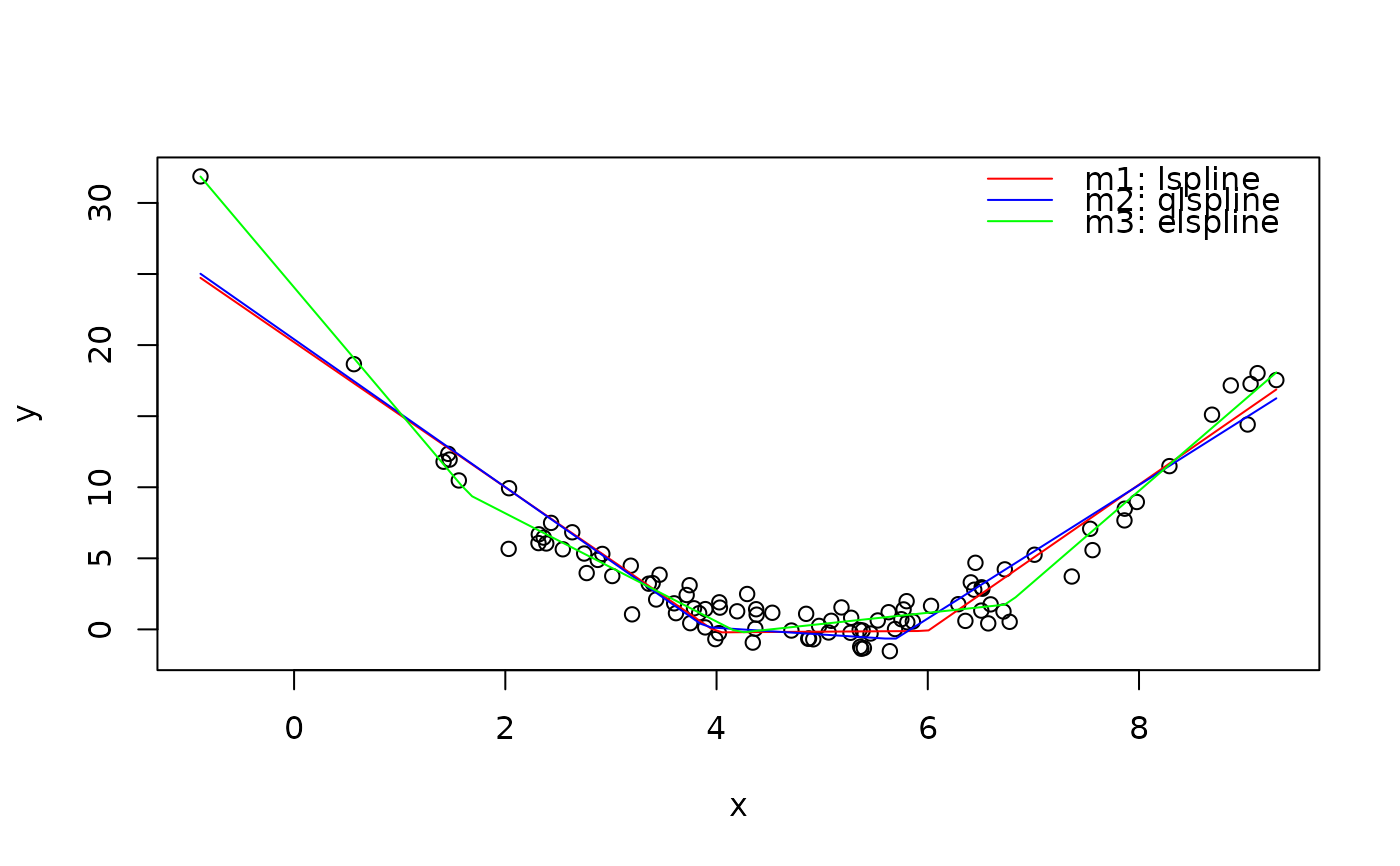
Basis for a piecewise linear spline with meaningful coefficients

These functions compute the basis of piecewise-linear spline such that, depending on the argument marginal, the coefficients can be interpreted as (1) slopes of consecutive spline segments, or (2) slope change at consecutive knots.

Usage

lspline(x, knots = NULL, marginal = FALSE, names = NULL)

qlspline(x, q, na.rm = FALSE, ...)

elspline(x, n, ...)

Arguments

x: numeric vector, the variable
knots: numeric vector of knot positions
marginal: logical, how to parametrize the spline, see Details
names: character, vector of names for constructed variables
q: numeric, a single scalar greater or equal to 2 for a number of equal-frequency intervals along x or a vector of numbers in (0; 1) specifying the quantiles explicitely.
na.rm: logical, whether NA should be removed when calculating quantiles, passed to na.rm of quantile.
...: other arguments passed to lspline
n: integer greater than 2, knots are computed such that they cut n equally-spaced intervals along the range of x

Details

If marginal is FALSE (default) the coefficients of the spline correspond to slopes of the consecutive segments. If it is TRUE the first coefficient correspond to the slope of the first segment. The consecutive coefficients correspond to the change in slope as compared to the previous segment.

Function qlspline wraps lspline and calculates the knot positions to be at quantiles of x. If q is a numerical scalar greater or equal to 2, the quantiles are computed at seq(0, 1, length.out = q + 1)[-c(1, q+1)], i.e. knots are at q-tiles of the distribution of x. Alternatively, q can be a vector of values in [0; 1] specifying the quantile probabilities directly (the vector is passed to argument probs of quantile).

Function elspline wraps lspline and computes the knot positions such that they cut the range of x into n equal-width intervals.

References

Poirier, Dale J., and Steven G. Garber. (1974) "The Determinants of Aerospace Profit Rates 1951-1971." Southern Economic Journal: 228-238.
Greene, William H. (2003) Econometric analysis. Pearson Education
Junger & Ponce de Leon (2011) "ares: Environment air pollution epidemiology: a library for timeseries analysis". R package version 0.7.2 retrieved from CRAN archives.

Author

This function is inspired by Stata command mkspline and function ares::lspline from Junger & Ponce de Leon (2011). As such, the implementation follows Greene (2003), chapter 7.2.5

Examples

# Data from a quadratic polynomial
set.seed(666)
x <- rnorm(100, 5, 2)
y <- (x-5)^2 + rnorm(100)
plot(x, y)

# -- Marginal and non-marginal parametrisations
m.nonmarginal <- lm(y ~ lspline(x, 5))
m.marginal <- lm(y ~ lspline(x, 5, marginal=TRUE))
# Slope of consecutive segments
coef(m.nonmarginal)
#>    (Intercept) lspline(x, 5)1 lspline(x, 5)2 
#>      18.125666      -4.211405       4.318447 
# Slope change and consecutive knots
coef(m.marginal)
#>                     (Intercept) lspline(x, 5, marginal = TRUE)1 
#>                       18.125666                       -4.211405 
#> lspline(x, 5, marginal = TRUE)2 
#>                        8.529853 
# Identical predicted values
identical( fitted(m.nonmarginal), fitted(m.marginal))
#> [1] FALSE


# -- Different ways to place knots
# Manually: knots at x=4 and x=6
m1 <- lm(y ~ lspline(x, c(4, 6)))
# 2 knots at terciles of 'x'
m2 <- lm(y ~ qlspline(x, 3))
# 3 knots dividing range of 'x' into 4 equal-width intervals
m3 <- lm(y ~ elspline(x, 4))

# Graphically
ox <- seq(min(x), max(x), length=100)
lines(ox, predict(m1, data.frame(x=ox)), col="red")
lines(ox, predict(m2, data.frame(x=ox)), col="blue")
lines(ox, predict(m3, data.frame(x=ox)), col="green")
legend("topright",
  legend=c("m1: lspline", "m2: qlspline", "m3: elspline"),
  col=c("red", "blue", "green"),
  bty="n", lty=1)