Network Segregation and Homophily

The following vignette demonstrates using the functions from package netseg (Bojanowski 2021). Two example datasets are described in the next section. Mixing matrices are described in section 2 and the measures are described in section 3. Please consult Bojanowski and Corten (2014) for further details.

Data

data(Classroom)

In the examples below we will use data Classroom, a directed network in a classroom of 26 kids (Dolata, n.d.). Ties correspond to nominations from a survey question “With whom do you like to play with?”. Here is a picture:

plot(
  Classroom,
  vertex.color = c("Skyblue", "Pink")[match(V(Classroom)$gender, c("Boy", "Girl"))],
  vertex.label = NA,
  vertex.size = 10,
  edge.arrow.size = .7
)
legend(
  "topright",
  pch = 21,
  legend = c("Boy", "Girl"),
  pt.bg = c("Skyblue", "Pink"),
  pt.cex = 2,
  bty = "n"
)

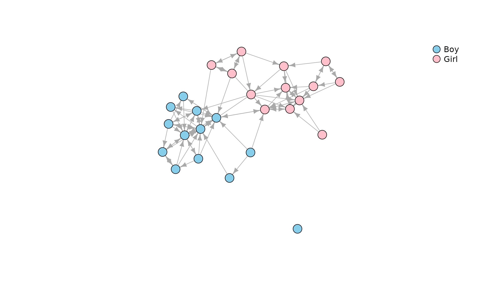
For us it will be a graph \(G = <V, E>\) where the node-set \(V = \{1, ..., i, ..., N\}\) correspond to kids, and edges \(E\) correspond to “play-with” nominations. Additionally, we need a node attribute, say \(X\), exhaustivelty assigning nodes to mutually-exclusive \(K\) groups. In the classroom example \(X\) is gender with values “Boy” and “Girl” (so \(K=2\)).

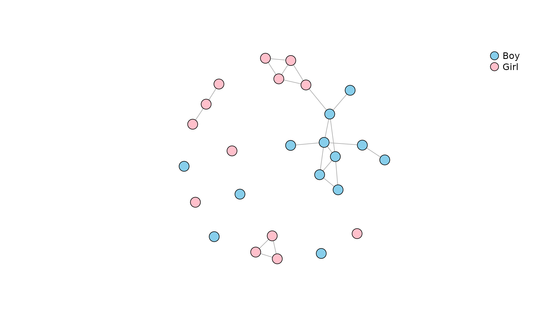
Some measures are applicable only to an undirected network. For that purpose let’s create an undirected network of reciprocated nominations in the Classroom network and call it undir:

undir <- as.undirected(Classroom, mode="mutual")
plot(
  undir,
  vertex.color = c("Skyblue", "Pink")[match(V(undir)$gender, c("Boy", "Girl"))],
  vertex.label = NA,
  vertex.size = 10,
  edge.arrow.size = .7
)
legend(
  "topright",
  pch = 21,
  legend = c("Boy", "Girl"),
  pt.bg = c("Skyblue", "Pink"),
  pt.cex = 2,
  bty = "n"
)

Mixing matrix

Mixing matrix is traditionally a two-dimensional cross-classification of edges depending on group membership of the adjacent nodes. A three-dimensional version of a mixing matrix cross-classifies all the dyads according to the following criteria:

Group membership of the ego
Group membership of the alter
Whether or not ego and alter are directly connected

Formally, mixing matrix is a matrix \(M\) in which entry \(m_{ghy}\) is a number of pairs of nodes such that

The first node belongs to group \(g\)
The second node belongs to group \(h\)
\(y\) is TRUE if there is a tie, \(y\) is FALSE if there is no tie

We can compute the mixing matrix for the classroom network and attribute gender with the function mixingm(). By default the traditional two-dimensional version is returned:

mixingm(Classroom, "gender")
#>       alter
#> ego    Boy Girl
#>   Boy   40    2
#>   Girl   5   41

Among other things we see that:

There are \(40 + 41 = 81\) ties within groups.
There are only \(5 + 2 = 7\) ties between groups.

Supplying argument full=TRUE the function will return an three-dimensional array cross-classifying the dyads:

m <- mixingm(Classroom, "gender", full=TRUE)
m
#> , , tie = FALSE
#> 
#>       alter
#> ego    Boy Girl
#>   Boy  116  167
#>   Girl 164  115
#> 
#> , , tie = TRUE
#> 
#>       alter
#> ego    Boy Girl
#>   Boy   40    2
#>   Girl   5   41

We can analyze the mixing matrix as a typical frequency crosstabulation. For example:

What is the probability of a tie depending on attributes of nodes?

round( prop.table(m, c(1,2)) * 100, 1)
#> , , tie = FALSE
#> 
#>       alter
#> ego     Boy Girl
#>   Boy  74.4 98.8
#>   Girl 97.0 73.7
#> 
#> , , tie = TRUE
#> 
#>       alter
#> ego     Boy Girl
#>   Boy  25.6  1.2
#>   Girl  3.0 26.3

What is the distribution of group memberships of alters depending on the attribute of ego?

round( prop.table(m[,,2], 1 ) * 100, 1)
#>       alter
#> ego     Boy Girl
#>   Boy  95.2  4.8
#>   Girl 10.9 89.1

In other words, boys are 95% of nominations of other boys, but only 11% of nominations of girls.

Function mixingm() works also for undirected networks, values below the diagonal are always 0:

mixingm(undir, "gender")
#>       ego
#> alter  Boy Girl
#>   Boy   11    1
#>   Girl   0   10
mixingm(undir, "gender", full=TRUE)
#> , , tie = FALSE
#> 
#>       ego
#> alter  Boy Girl
#>   Boy   67  168
#>   Girl   0   68
#> 
#> , , tie = TRUE
#> 
#>       ego
#> alter  Boy Girl
#>   Boy   11    1
#>   Girl   0   10

Most of the segregation indexes described below summarize the mixing matrix.

Mixing data frames

Function mixingdf() returns the same data in the form of a data frame. For directed Classroom network:

mixingdf(Classroom, "gender")
#>    ego alter  n
#> 1  Boy   Boy 40
#> 2 Girl   Boy  5
#> 3  Boy  Girl  2
#> 4 Girl  Girl 41
mixingdf(Classroom, "gender", full=TRUE)
#>    ego alter   tie   n
#> 1  Boy   Boy FALSE 116
#> 2 Girl   Boy FALSE 164
#> 3  Boy  Girl FALSE 167
#> 4 Girl  Girl FALSE 115
#> 5  Boy   Boy  TRUE  40
#> 6 Girl   Boy  TRUE   5
#> 7  Boy  Girl  TRUE   2
#> 8 Girl  Girl  TRUE  41

For undir:

mixingdf(undir, "gender")
#>   alter  ego  n
#> 1   Boy  Boy 11
#> 3   Boy Girl  1
#> 4  Girl Girl 10
mixingdf(undir, "gender", full=TRUE)
#>   alter  ego   tie   n
#> 1   Boy  Boy FALSE  67
#> 3   Boy Girl FALSE 168
#> 4  Girl Girl FALSE  68
#> 5   Boy  Boy  TRUE  11
#> 7   Boy Girl  TRUE   1
#> 8  Girl Girl  TRUE  10

Measures

Assortativity coefficient

assort(Classroom, "gender")
#> [1] 0.8408885
assort(undir, "gender")
#> [1] 0.9089027

Coleman’s homophily index

Coleman’s index compares the distribution of group memberships of alters with the distribution of group sizes. It captures the extent the nominations are “biased” due to the preference for own group.

We have a separate value for each group
Values are in [-1; 1]
- 0 – Members of the given group nominate their group peers proportionally to the relative group size.
- 1 – All nominations are from own group.
- -1 – All nominations are from groups other than own.

coleman(Classroom, "gender")
#>       Boy      Girl 
#> 0.9084249 0.7909699

Values are close to 1 (high segregation). The value for boys is greater than for girls, so girls nominated boys a bit more often than boys nominated girls.

E-I

ei(Classroom, "gender")
#> [1] -0.8409091
ei(undir, "gender")
#> [1] -0.9090909

Freeman’s segregation index

Is applicable to undirected networks with two groups.

Values in [0;1]

Function freeman:

freeman(undir, "gender")
#> [1] 0.9125874

Gupta-Anderson-May

gamix(Classroom, "gender")
#> [1] 0.9058693
gamix(undir, "gender")
#> [1] 0.8257576

Odds-ratio

orwg(Classroom, "gender")
#> [1] 16.58071
orwg(undir, "gender")
#> [1] 26.13333

Segregation Matrix Index

smi(Classroom, "gender")
#>       Boy      Girl 
#> 0.9117647 0.9138241

Spectral segregation index

Values for vertices

(v <- ssi(undir, "gender"))
#>         1         2         3         4         5         6         7         8 
#> 1.1392193 0.7033670 0.9816498 1.0000000 1.0000000 0.9973715 1.0000000 0.0000000 
#>         9        10        11        12        13        14        15        16 
#> 0.0000000 0.0000000 0.0000000 0.0000000 0.7151930 0.6925726 0.0000000 1.0333177 
#>        17        18        19        20        21        22        23        24 
#> 0.9701057 1.0344291 1.0550505 1.0299471 1.0000000 1.0000000 1.0000000 1.1031876 
#>        25        26 
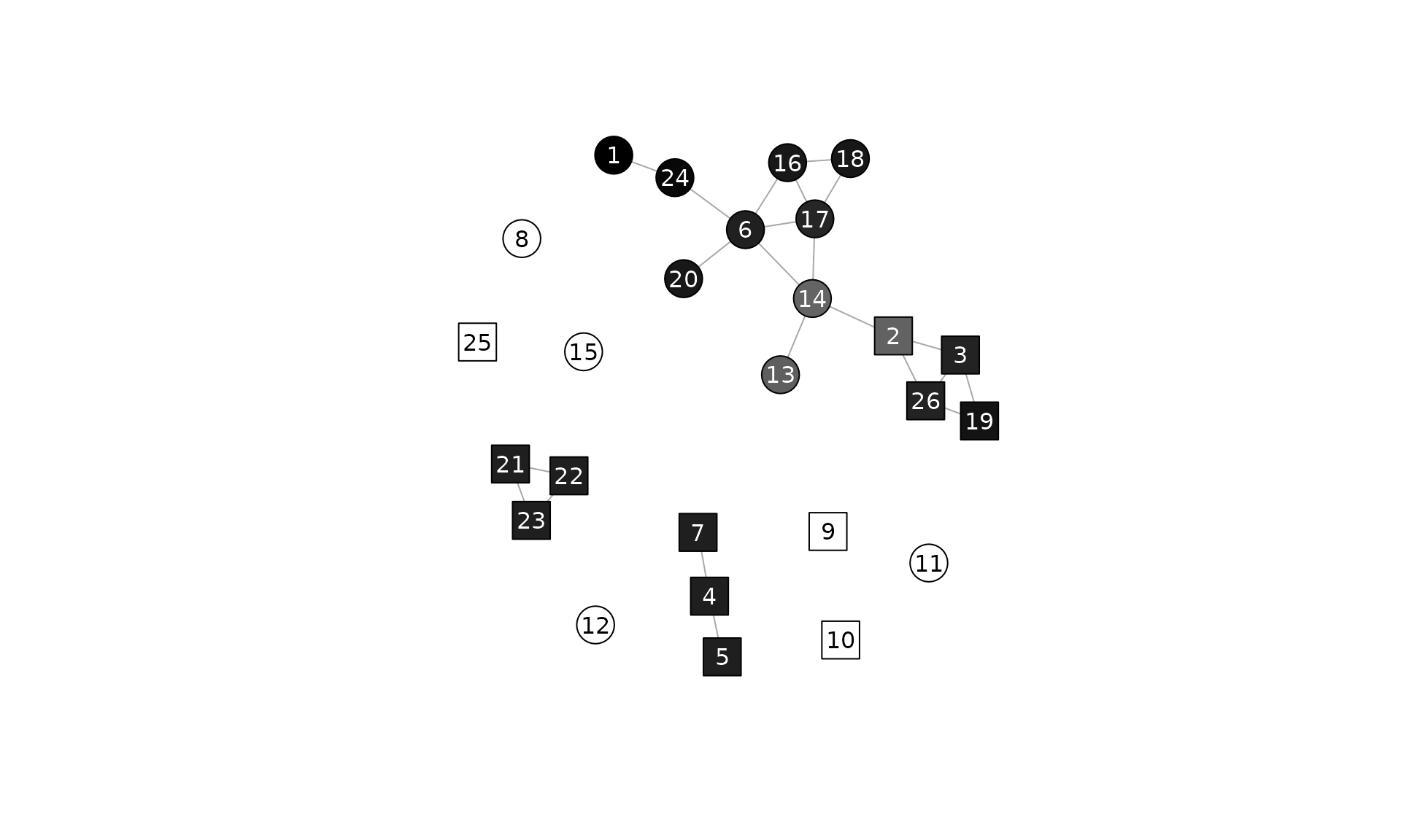
#> 0.0000000 0.9816498

Plotted with grayscale (the more segregated the darker the color):

kol <- gray(scales::rescale(v, 1:0))
plot(
  undir,
  vertex.shape = c("circle", "square")[match(V(undir)$gender, c("Boy", "Girl"))],
  vertex.color = kol,
  vertex.label = V(undir),
  vertex.label.color = ifelse(apply(col2rgb(kol), 2, mean) > 125, "black", "white"),
  vertex.size = 15,
  vertex.label.family = "sans",
  edge.arrow.size = .7
)

References

Bojanowski, Michał. 2021. Measures of Network Segregation and Homophily. https://mbojan.github.io/netseg/.

Bojanowski, Michał, and Rense Corten. 2014. “Measuring Segregation in Social Networks.” Social Networks 39: 14–32. https://doi.org/10.1016/j.socnet.2014.04.001.

Dolata, Roman, ed. n.d. Czy Szkoła Ma Znaczenie? Zróżnicowanie Wyników Nauczania Po Pierwszym Etapie Edukacyjnym Oraz Jego Pozaszkolne i Szkolne Uwarunkowania. Vol. 1. Warsaw: Instytut Badań Edukacyjnych.

Michał Bojanowski

February 15, 2021